Lab 2: Inertial Measurement Unit
Setting up the IMU
I began by connecting the IMU to the Artemis. After flashing the example code, I was able to display real time values from the accelerometer.I set AD0_VAL to 1 to define the I2C address of the IMU. In this case, without soldering any connections the board maintains the default address of 0x12.
Next, I checked the calibration of the sensor. The values seemed to be quite consistent, so I don't think a two-point calibration is neccessary.
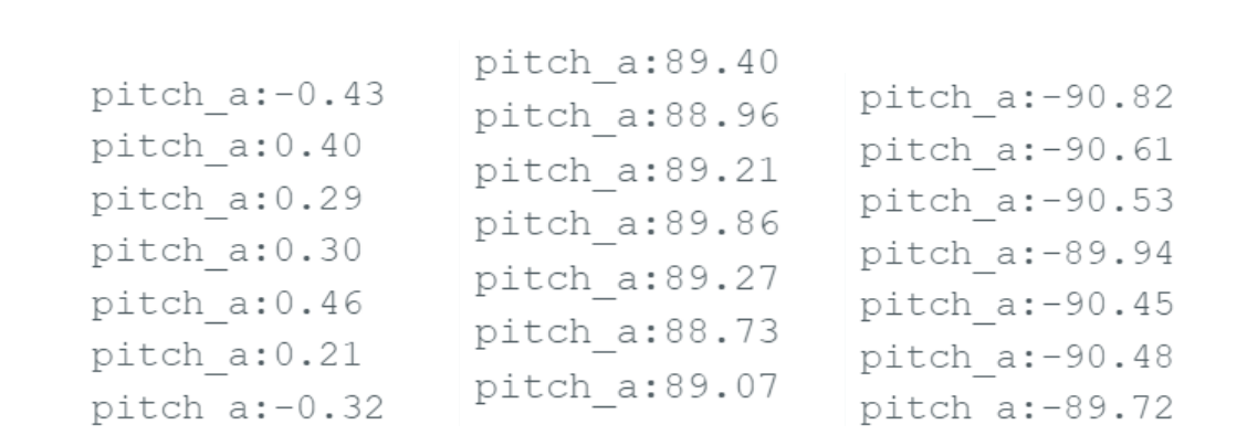
Pitch Calibration (measured at 0, 90, and -90 degrees)
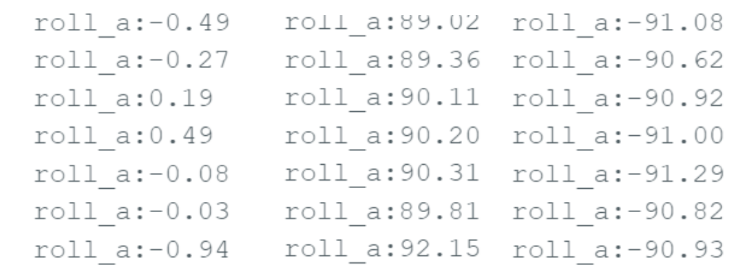
Roll Calibration (measured at 0, 90, and -90 degrees)
Accelerometer Data
I used the following code to calculate pitch and roll from accelerometer values:
if(myICM.dataReady())
    {
    myICM.getAGMT();
    currentMillis = millis();
    time_stamps[i] = currentMillis;

    //accel pitch
    pitch_a = atan2(myICM.accY(),myICM.accZ())*180/M_PI;
    pitch_a_array[i] = pitch_a;

    //accel roll
    roll_a = atan2(myICM.accX(),myICM.accZ())*180/M_PI;
    roll_a_array[i] = roll_a;
    }
I then appended the values to the string GAAT characteristic, utlilizing a notification handler to record the values in an array for plotting.
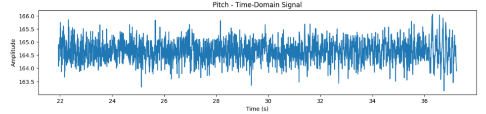
Plotted Pitch Data (static noise)
The data looked very noisy on all axes. To address this, I took a fourier transform of the data to better understand the frequency spectrum that contained the noise.
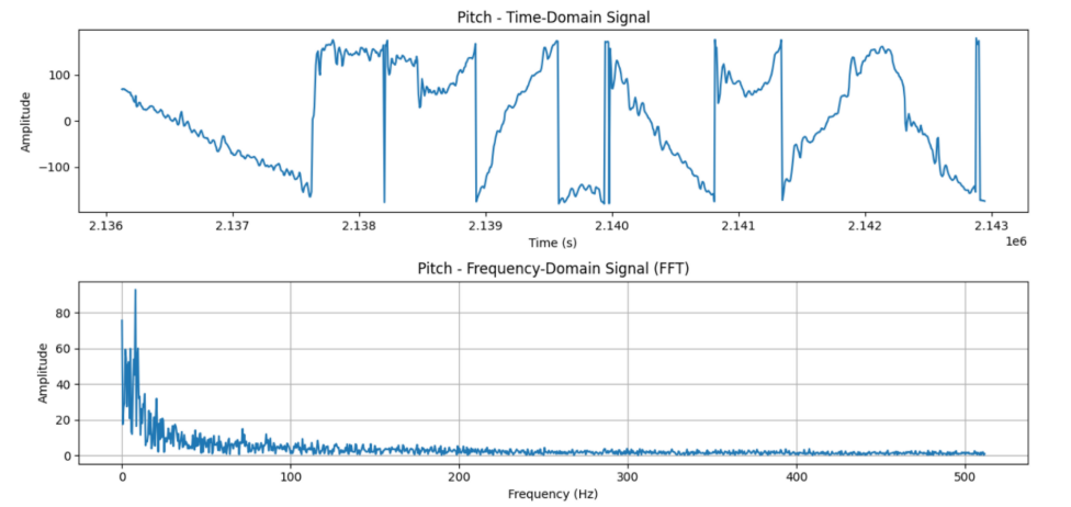
In the frequency domain, most of the notable spikes appear between 0-5Hz. As such, I chose 5Hz as my cutoff frequency. I also calculated my data rate to be 129 messages/sec. With these numbers and the equations below, I calculated an alpha value of 0.15 for a low pass filter.
This number is important - too high and you will be removing information with your filter. However, too low will be ineffective for removing noise.
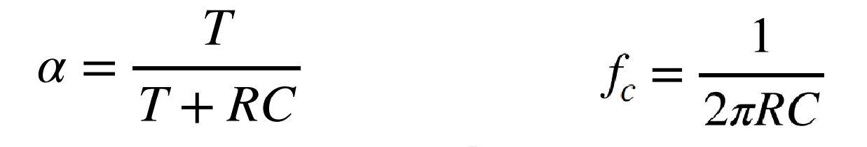
Where f_c is cutoff frequency and T is 1/sampling rate.
Using this calculated alpha value, I implemented a low pass filter for pitch and roll.
//accel pitch low pass filter
lpf_pitch_a_array[i] = alpha * pitch_a + (1 - alpha) * lpf_pitch_a_array[i - 1];
lpf_pitch_a_array[i - 1] = lpf_pitch_a_array[i];
The resulting signal is less susceptible to noise!
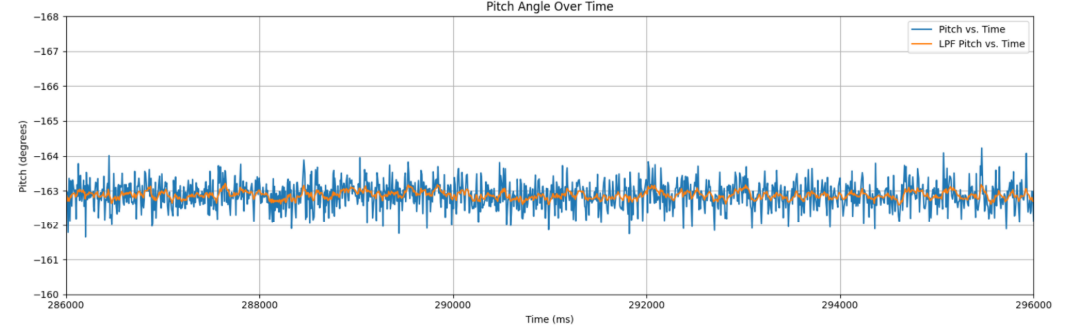
LPF, static noise
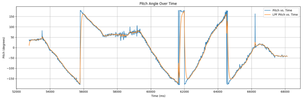
LPF, isolated circle motion
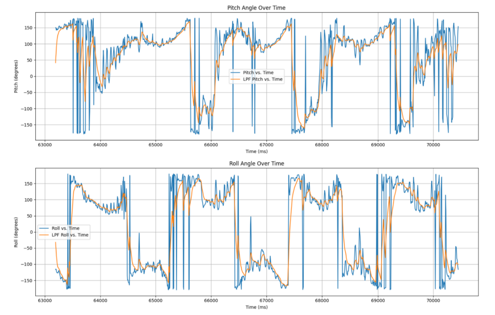
LPF, full circle motion. The raw signal is incredibly noisy, but the filter does a pretty good job at capturing the macro motion of the sensor.
Gyroscope Data
Next, I implemented data collection for the gyro sensor. Note that the X and Y axes had to be flipped to match the orientation of the gyro and accel sensors on the board.
//gyro pitch, roll, yaw
dt = (millis()-lastT)/1000.;
lastT = millis();

pitch_g_array[i] = pitch_g_array[i-1] + myICM.gyrX()*dt;
roll_g_array[i] = roll_g_array[i-1] - myICM.gyrY()*dt;
yaw_g_array[i] = yaw_g_array[i-1] + myICM.gyrZ()*dt;
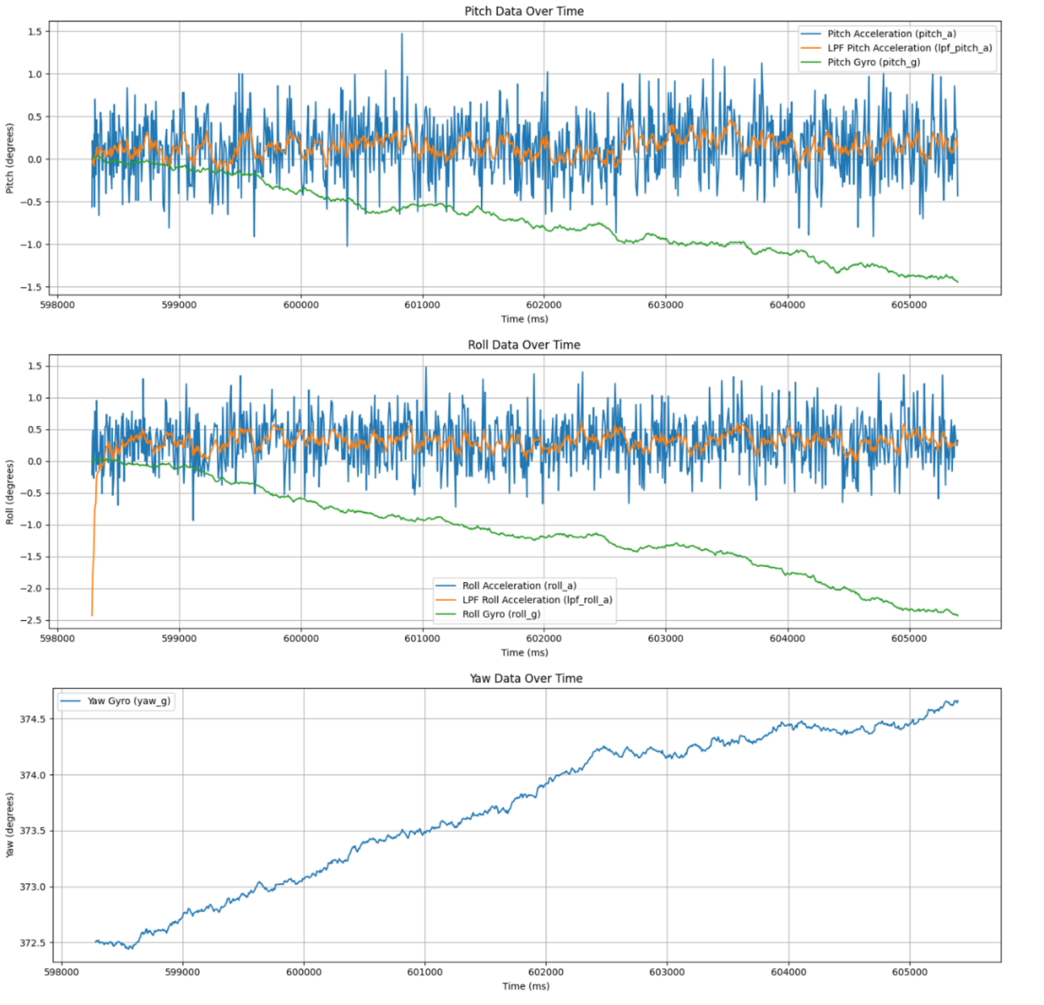
Gryo data compared to accelerometer. While the noise isn't as bad, there is drift due to integrating error over time. The accelerometer also seems to introduce lots of noise in an axis when measuring an acceleration in a different direction - the gyro is better at isolating measurements.
To deal with the drift, I implemented a complementary filter that used both sensors to achieve a more accurate measurement. I used the same alpha value from before, biasing the data towards the smooth gyro measurements.
//gyo complementary filter
comp_pitch_g_array[i] = ( comp_pitch_g_array[i-1] + myICM.gyrX()*dt ) * (1 - alpha) + (alpha*lpf_pitch_a_array[i]);
comp_roll_g_array[i] = ( comp_roll_g_array[i-1] - myICM.gyrY()*dt ) * (1 - alpha) + (alpha*lpf_roll_a_array[i]);
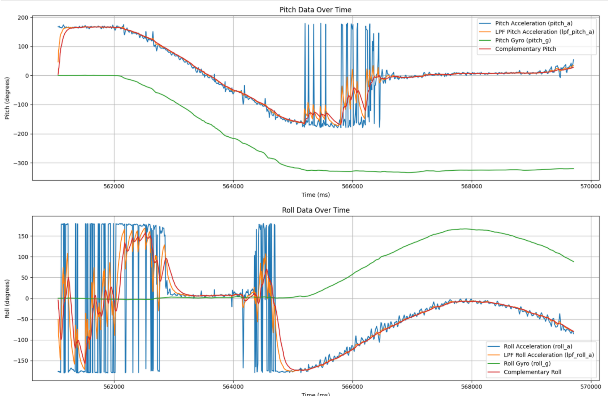
Comparing signals for a slow rotation. Note the lack of drift in the complementary signal.
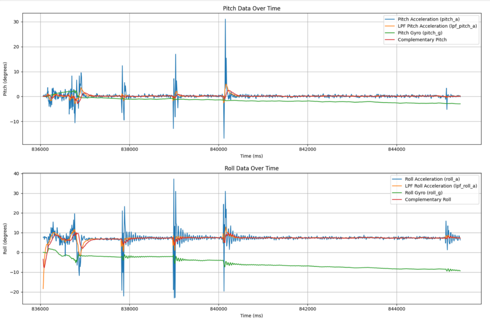
Sensor data in response to sudden vibrations. The complementary signal doesn't drift like the gryo data, and is also a bit less susceptible to vibration when compared to the accelerometer data. In many ways, this filter retains the best characteristics of each sensor.
Data Sampling
After removing all print statements, I was able to get up to around 130 messages/sec. I used floats for all of the data, as the decimal value made sense for the type of data I was collecting. I didn't use doubles because they take up more space than a float, and I didn't need the extra precision. I used 10 arrays in total - 1 time array, 4 accelerometer data arrays (including filtered data), and 5 gyroscope data arrays. Consolidating this data into less arrays might be more memory efficient, but I found that splitting the data up this way made the parsing further down the line much more organized and readable.
With this setup, I was able to achieve 17 seconds of data by making each array 5000 data points long. I was able to increase this length all the way to 8000 before reaching memory problems, implying a max data collection time of almost 30 seconds.
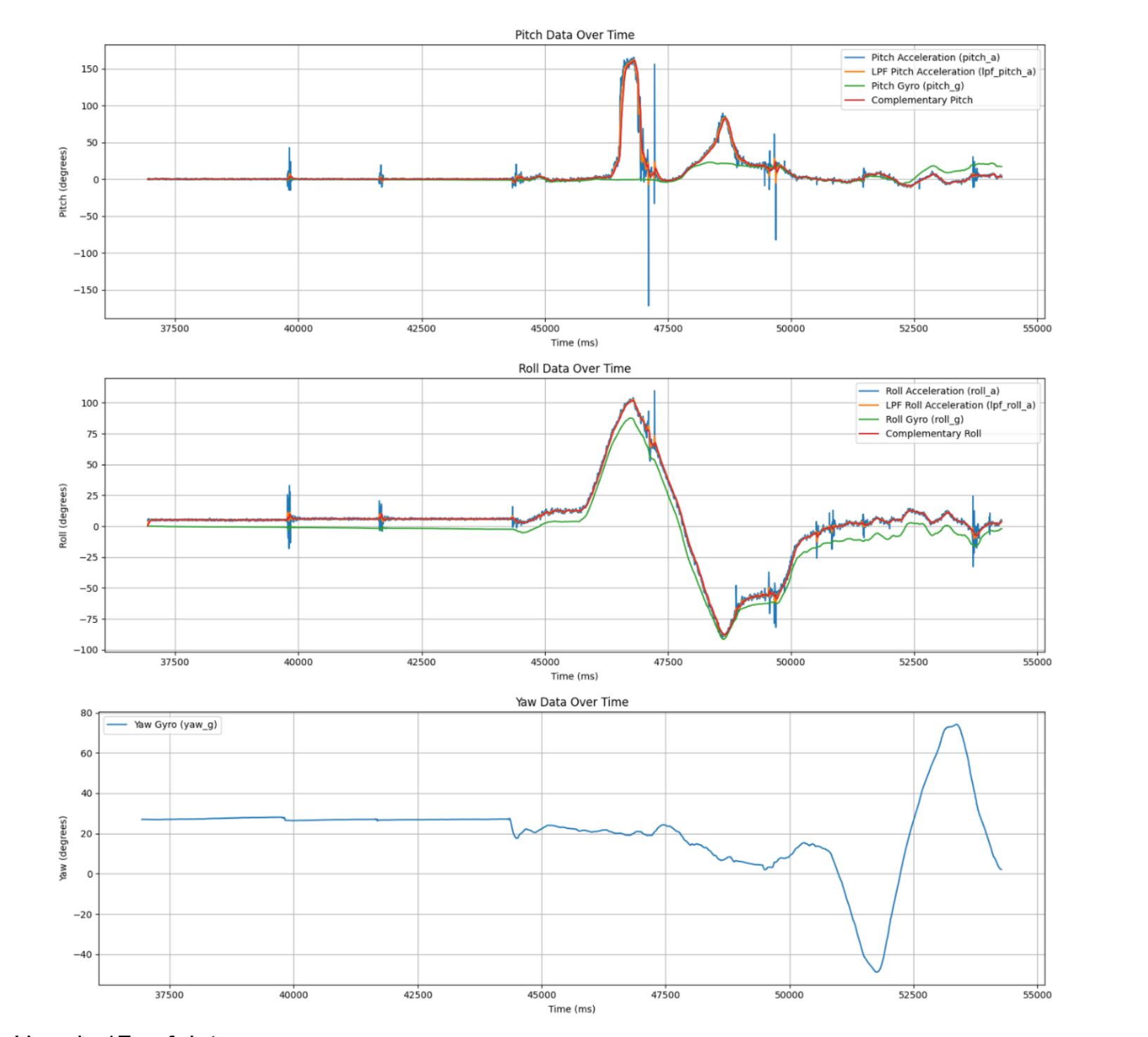
17 seconds of data.
Car Stunt
This week, we received our cars! I was able to get it to flip by quickly decelerating the car. One thing to note is the absolute lack of fine control.
Collaboration
I worked with Jack Long and Lucca Correia extensively. I also referenced both Daria's website and Nila's website from last year for help implementing some of the filters. Lastly, I utilized ChatGPT for lots of error debugging, and also to speed up writing plotting syntax.