Establishing the Time of Flight (TOF) sensor

The robot will use two TOF sensors to collect data from the environment. I decided to mount one sensor on the front of the car for obstacle detection in the path of motion. I will put the other sensor on the side of the car, primarily for improved mapping and the ability to drive along a wall. A potential weakness is an inability to see behind the robot.

In order to use two sensors with the same address, I used the XSHUT pin on a sensor to shut it off momentarily. I modified the address of the other sensor, and was then able to reinitialize the orignal sensor. After this, the sensors can function at the same time.

digitalWrite(SHUTDOWN_PIN, LOW); // Shut down TOF2
distanceSensor1.begin();
distanceSensor1.setI2CAddress(0xf5);
distanceSensor1.begin()
distanceSensor1.setDistanceModeShort();
digitalWrite(SHUTDOWN_PIN, HIGH); // Restart TOF2 
distanceSensor2.begin() 
distanceSensor2.setDistanceModeShort();

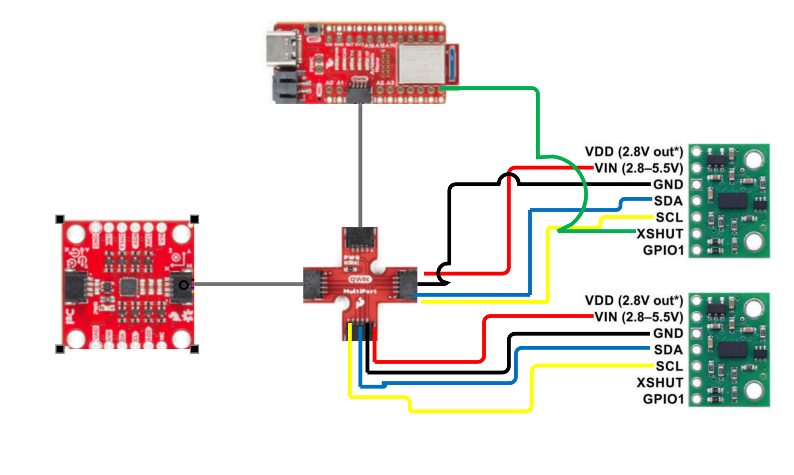
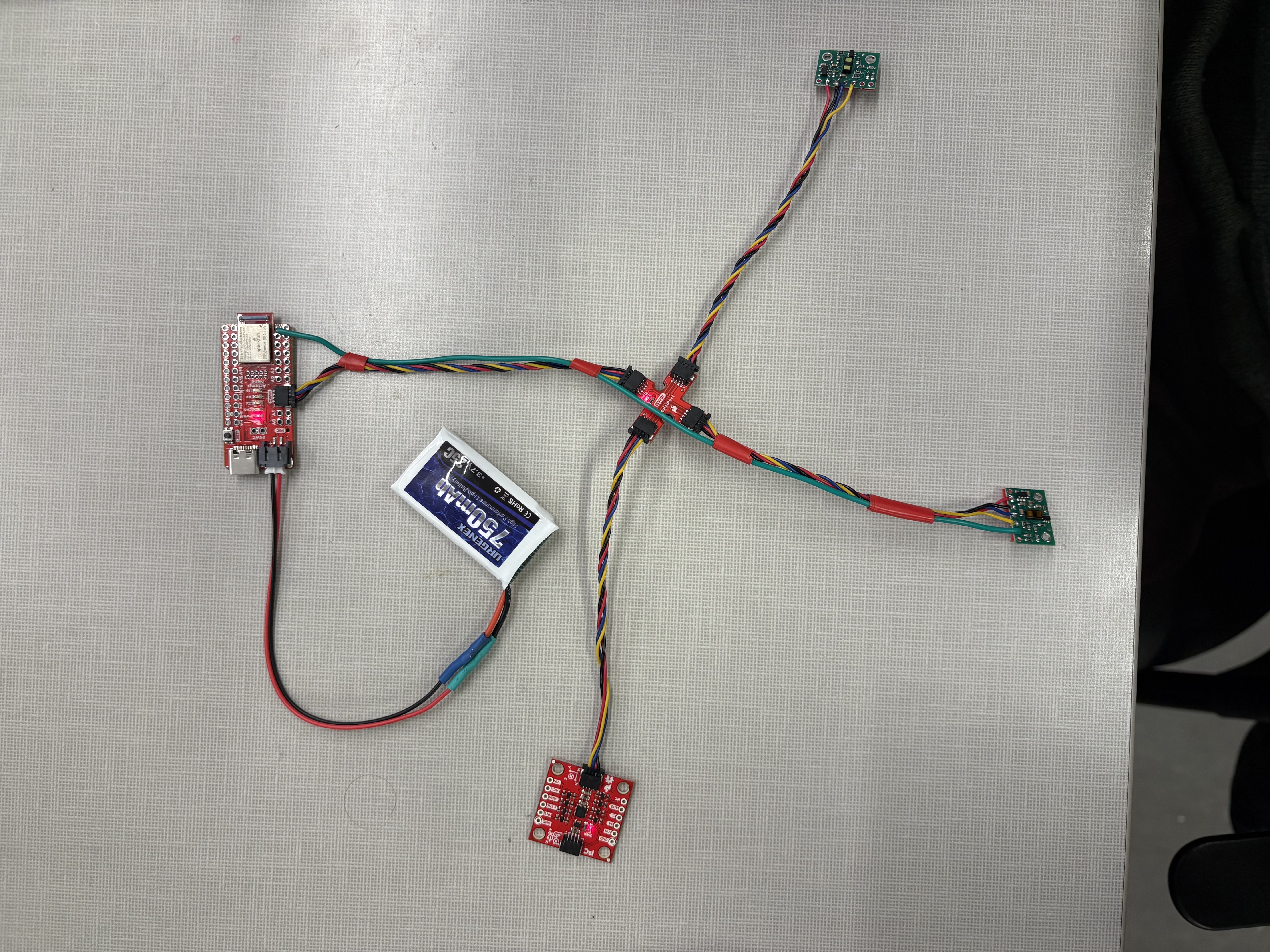
Wiring Diagram

Next, I soldered the connection and was able to establish a bluetooth connection with the electronics being powered by the battery.

Characterizing the TOF sensor

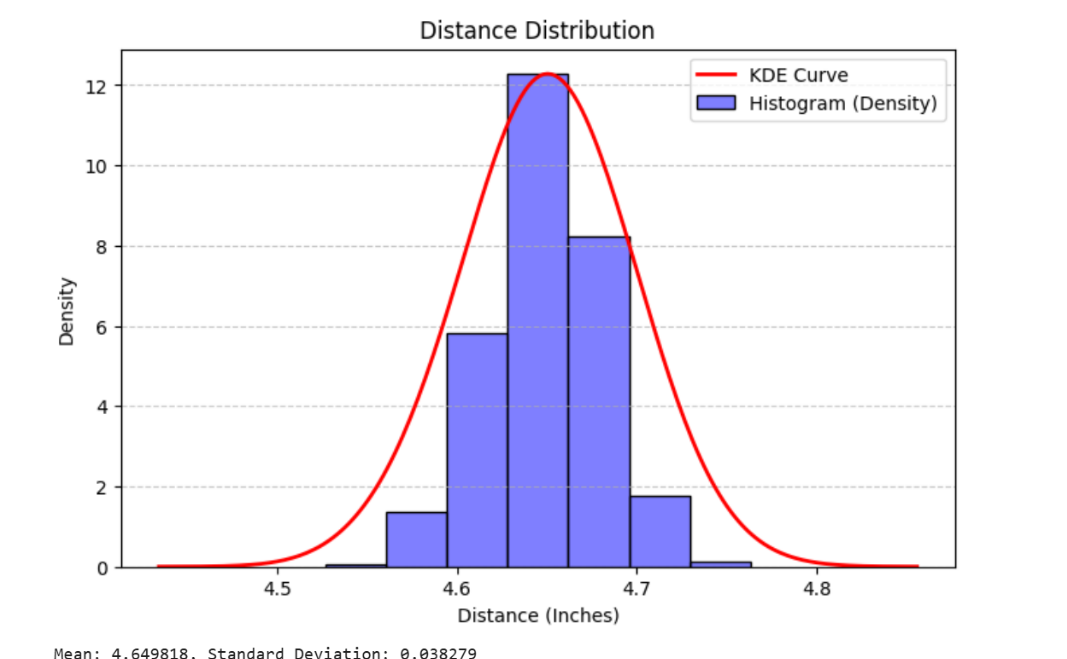
I next investigated the consistency and accuracy of the data being collected. I measured out a 5 inch gap and secured the sensor this far from a white cardboard box. I then collected 500 data points to get an idea of what the noise profile of the sensor looked like.

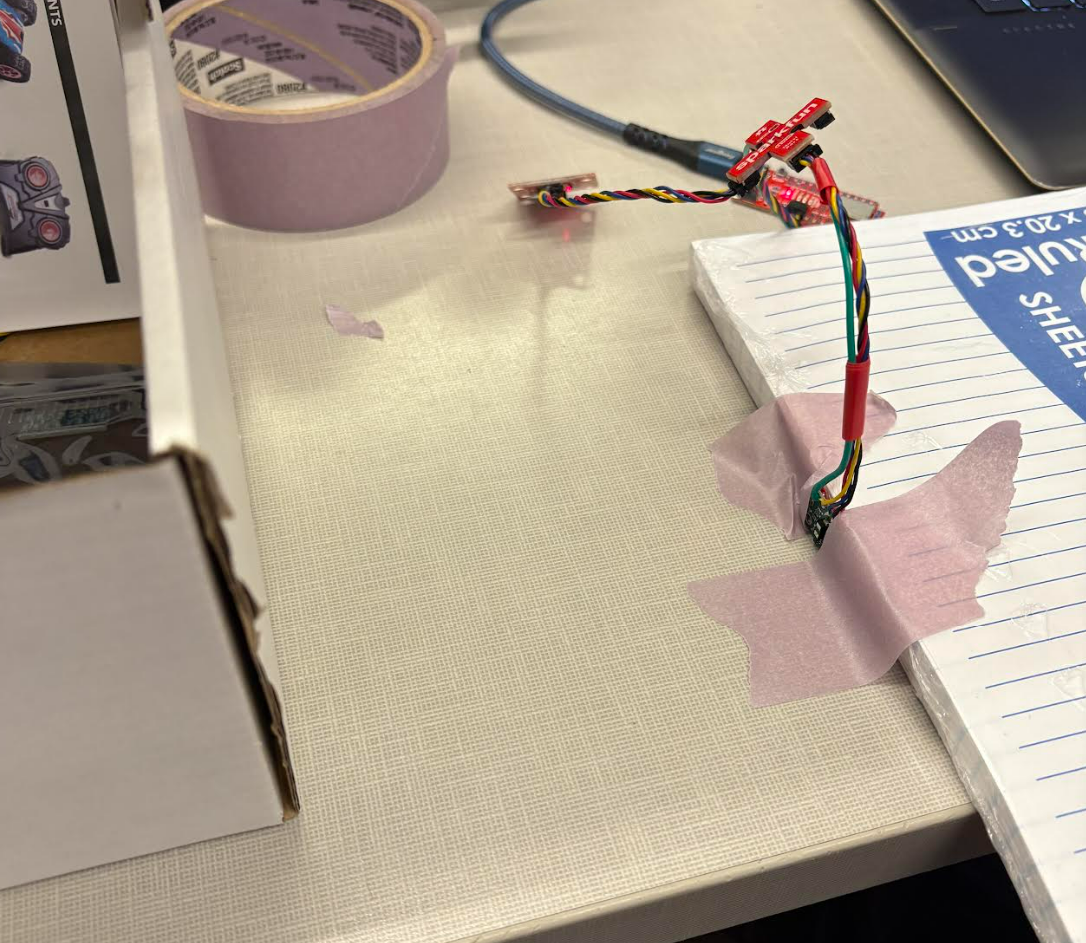
TOF sensor secured 5 inches from object. The gap was measured with a tape measure.

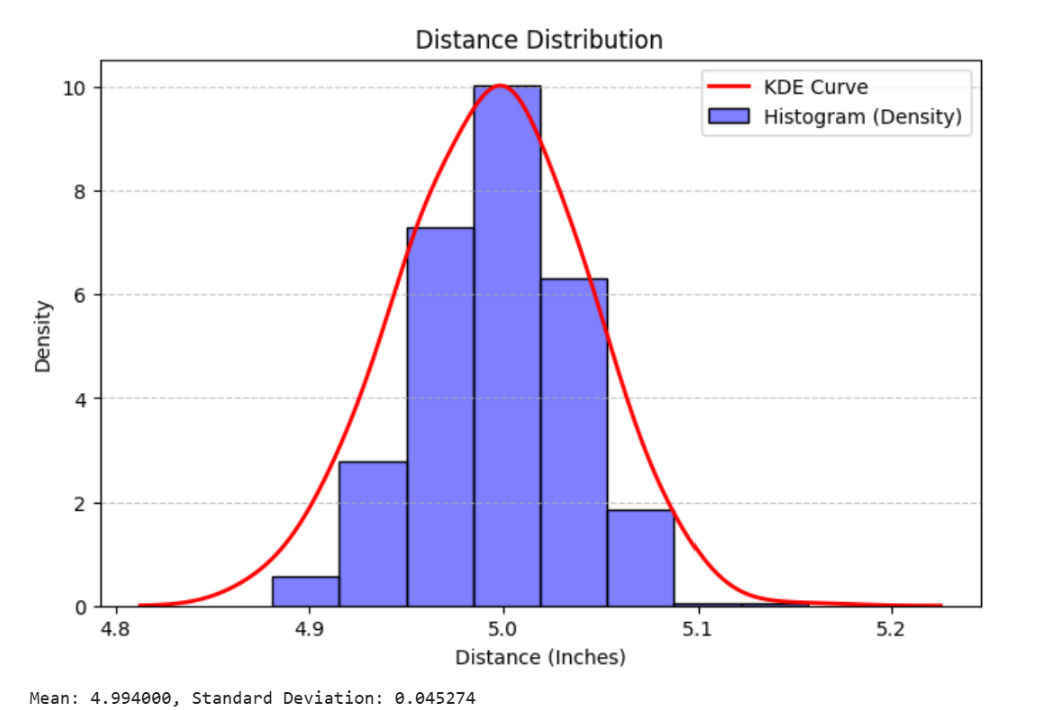
Measurement distribution, short mode

Measurement distribution, long mode

I repeated this trial at 20 inches with pretty similar results. My take away from this is that both modes have pretty similar noise profiles, but short mode gets closer to the true distance measurment. For this reason, I'm going to use short mode going forward unless I run into issues at much longer ranges - short mode seemed to work fine for distances under about 4 feet. Otherwise, it's nice to see that the large majority of data points fall within a ~0.1" spread.

Another note from these trials is that the resolution of the measurement is not as high as I initially thought. The number being collected is reported to a thousandth of an inch, but the sensor is not this high resolution. I inititally made the buckets in my histogram much smaller, and the resultant banding shows that the sensor is only reporting distance to the nearest 1/3 of an inch.

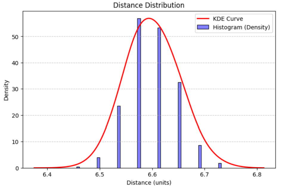
The large gaps between filled buckets in this histogram shows the lack of resolution in the sensor.

Considering speed with two sensors

With the wiring shown above, I was able to get both sensors collecting data at the same time.

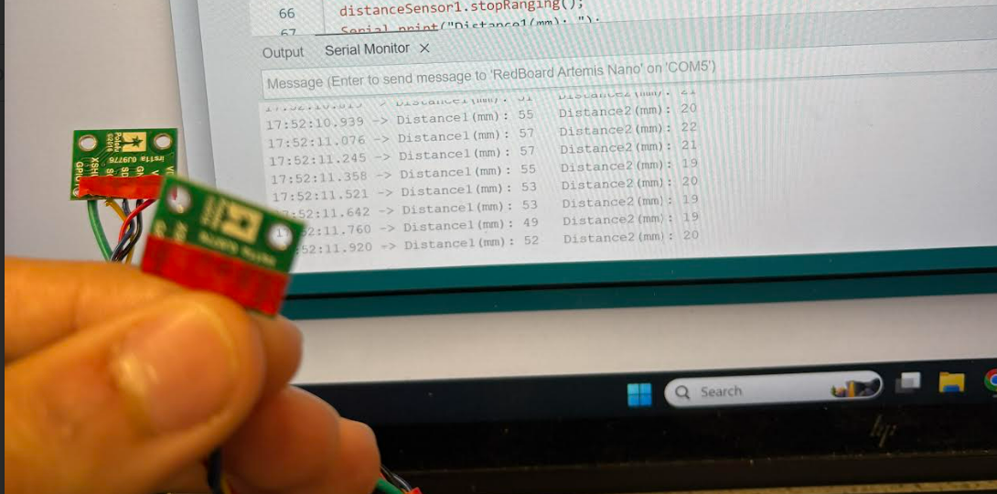
I then looped this code snipped to compare the sensor speed to the artemis clock speed:

distanceSensor1.startRanging();
distanceSensor2.startRanging();

if (distanceSensor1.checkForDataReady())
    {
    int distance1 = distanceSensor1.getDistance();
    distanceSensor1.clearInterrupt();
    distanceSensor1.stopRanging();
    Serial.print("Distance1: ");
    Serial.print(distance1);
    Serial.println("   ");
    }

if (distanceSensor2.checkForDataReady())
    {
    int distance2 = distanceSensor2.getDistance(); 
    distanceSensor2.clearInterrupt();
    distanceSensor2.stopRanging();
    Serial.print("Distance2: ");
    Serial.print(distance2);
    Serial.println("   ");
    }

Serial.print("T: ");
Serial.print(millis());
Serial.print("   ");
Serial.println();

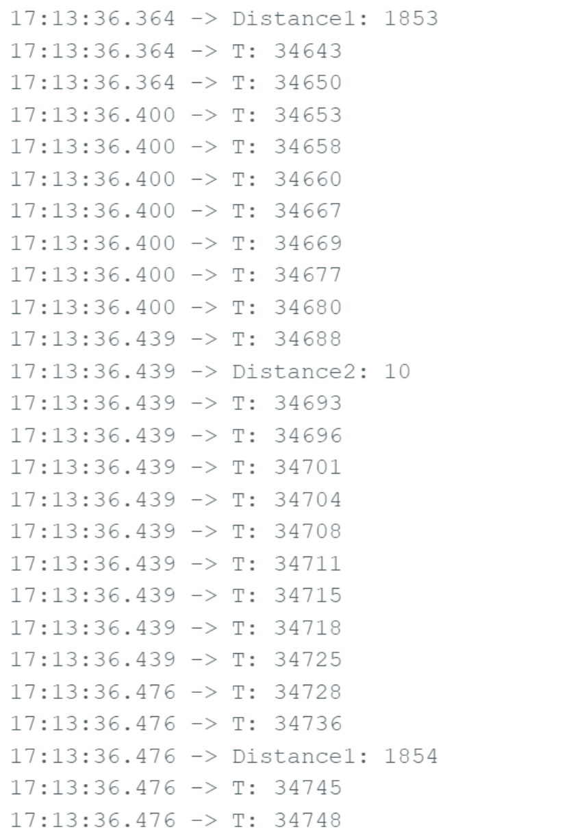
Result of running this code. The delay for each sensor seems to vary between 100-200ms, indicating a sampling rate of 5-10Hz. The Artemis clock is 20-30x faster than an individual sensor; the sensors just take a long time to have data ready.

Final implementiation and plotting

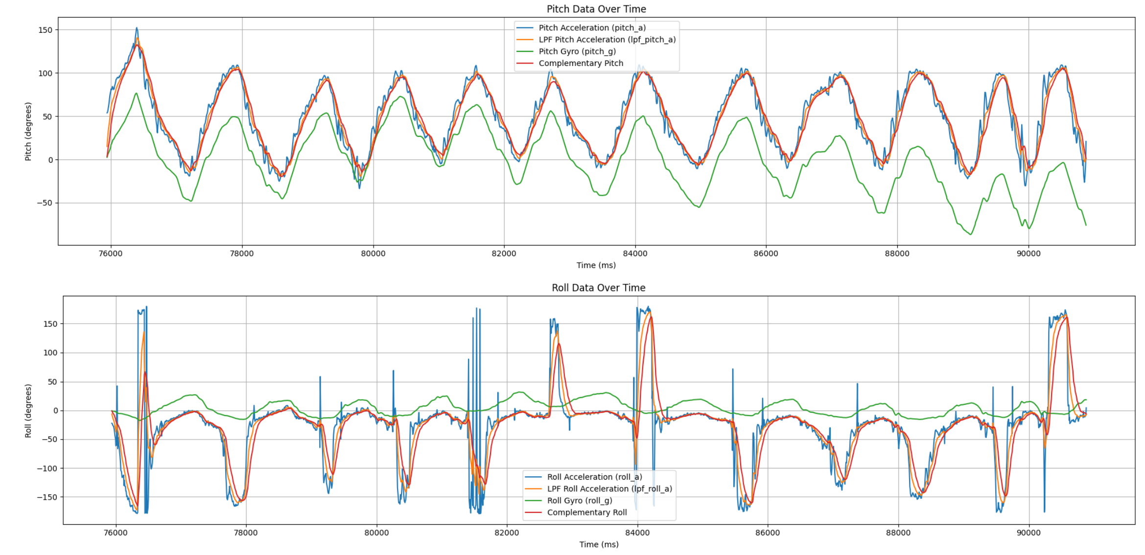
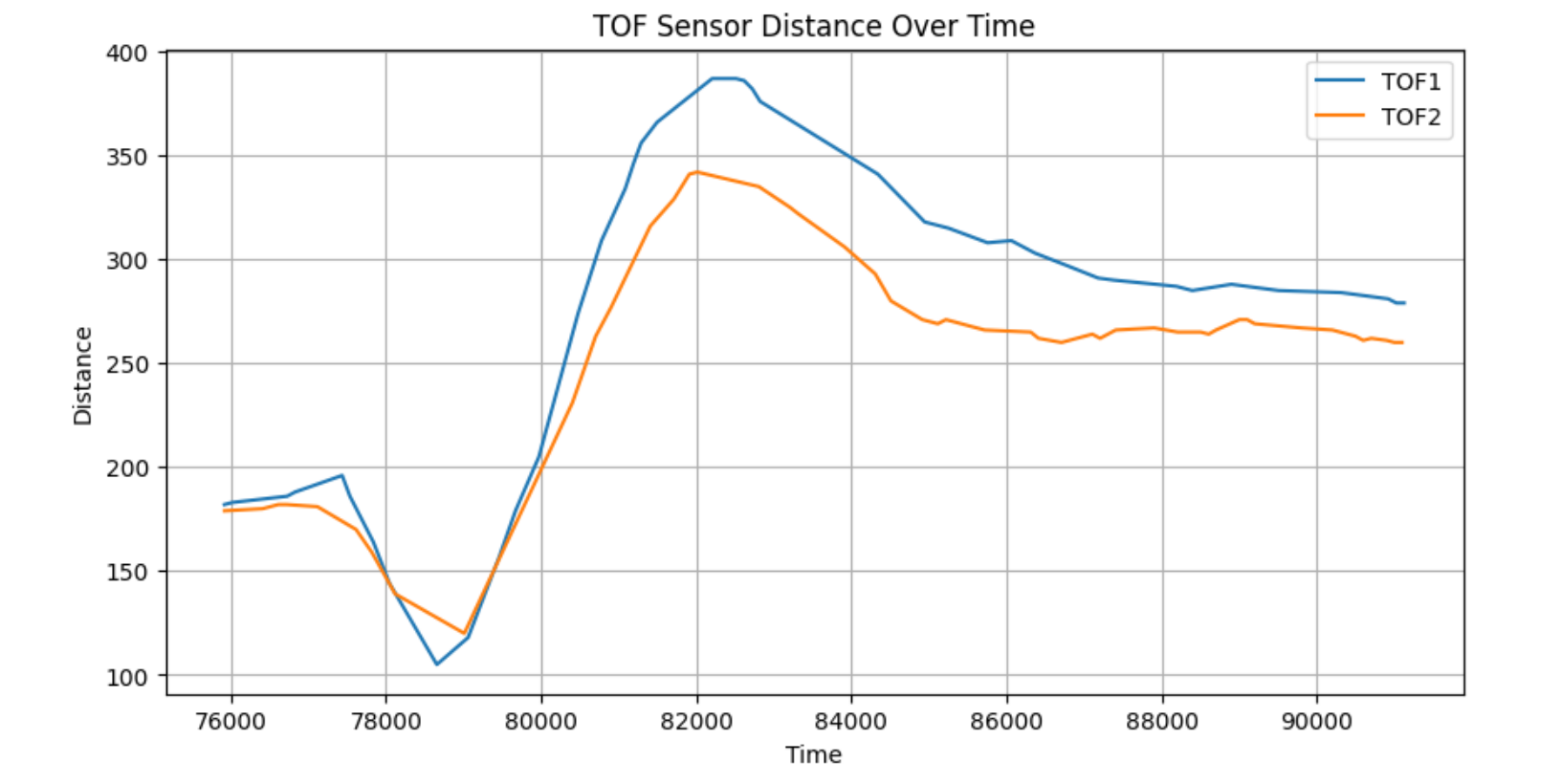
With all of my sensors now working, I next implemented functions in my Artemis code to collect data. By controlling whether these functions run using flags sent through commands, I have full control over when each sensor is active. Below are graphs of IMU and TOF data, all taken during the same time frame. It's worth noting that the sampling rate of the TOF sensors is much slower than the IMU.

Collaboration

I worked with Jack Long and Lucca Correia extensively. I also referenced Wenyi's website from last year for wiring and utilizing the XSHUT pin. Lastly, I used ChatGPT for error debugging and to speed up plotting.