Lab 7: Kalman Filtering
Estimating Mass and Drag
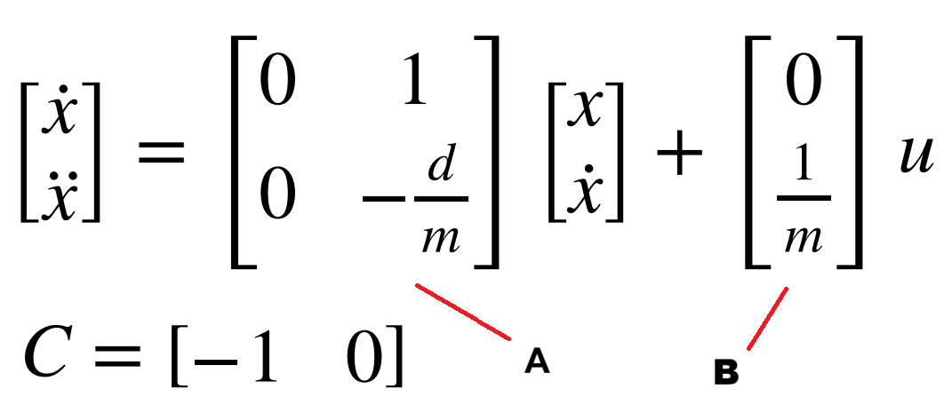
To build the state space model for my robot, I first needed to accurately estimate the mass and drag acting on my car. Following the derivation outlined in Farrell's Lecture 13, the dynamics of the system can be expressed as follows:
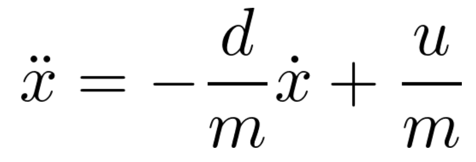
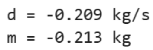
Now considering a step response from rest to a steady state velocity, acceleration is zero once this velocity is reached. The d and m terms can then be solved for:
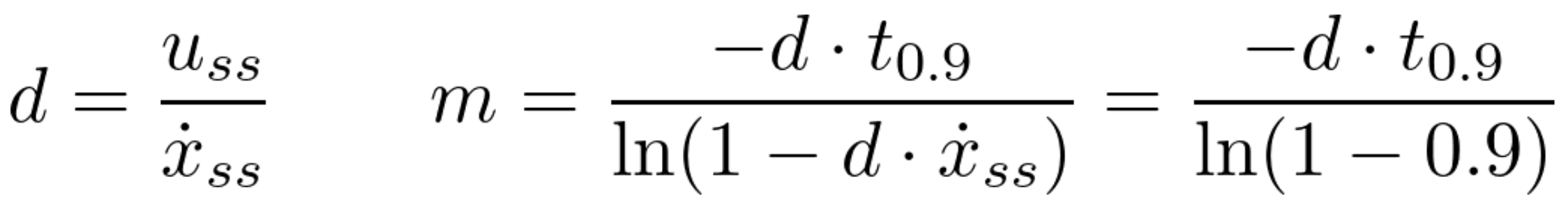
d and m are lumped parameters that capture the dynamics of the system - how the car responds to control inputs and moves through the world. uss is the constant control input being passed to the robot for this test. I decided to use an input of 1, corresponding to the maximum pwm signal possible (255). I did this because I wanted my dynamics to be accurate when my robot is moving quickly, as this is the ideal behavior of an accurate controller.
Step Response Test
With this TOF data, I was able to calculate the velocity at each time step:
# Compute velocity (finite difference method)
velocity_values = []
for i in range(len(tof2_time_values) - 1):  # Loop over indices
    if (tof2_time_values[i] == tof2_time_values[0]):
        dt = 1
        dd = .000001
    else:
        dt = tof2_time_values[i] - tof2_time_values[i-1]  # Time difference
        dd = tof2_values[i] - tof2_values[i-1]  # Distance difference

    velocity = dd / dt  # Velocity calculation
    velocity_values.append(round(velocity,3))

velocity_values.append(0) # ensure arrays of equal length
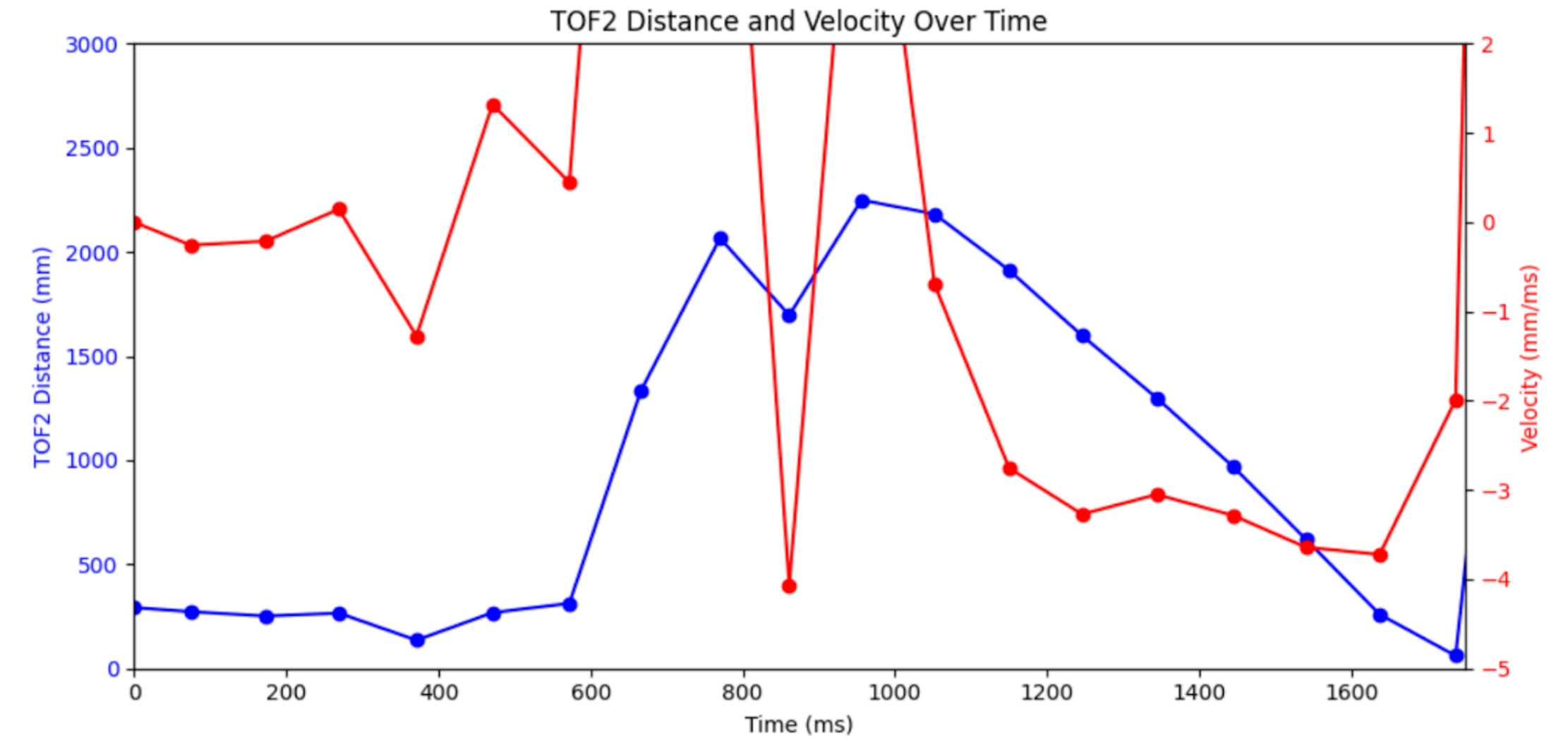
One problem I ran into is that my high step input meant that the robot needed to drive for a long distance in order to reach anywhere near its maximum speed. This was exacerbated by the fact that my front TOF only reliably worked up to 2000mm rather than the expected 4000mm.
My solution to this was to run multiple tests, starting from different distances to the wall. I then made the assumption that each test would have the same position and velocity curve shapes. Even though I would only get good readings under 2000mm from the wall, I was able to manually combine the data from multiple tests into one comprehensive position curve.
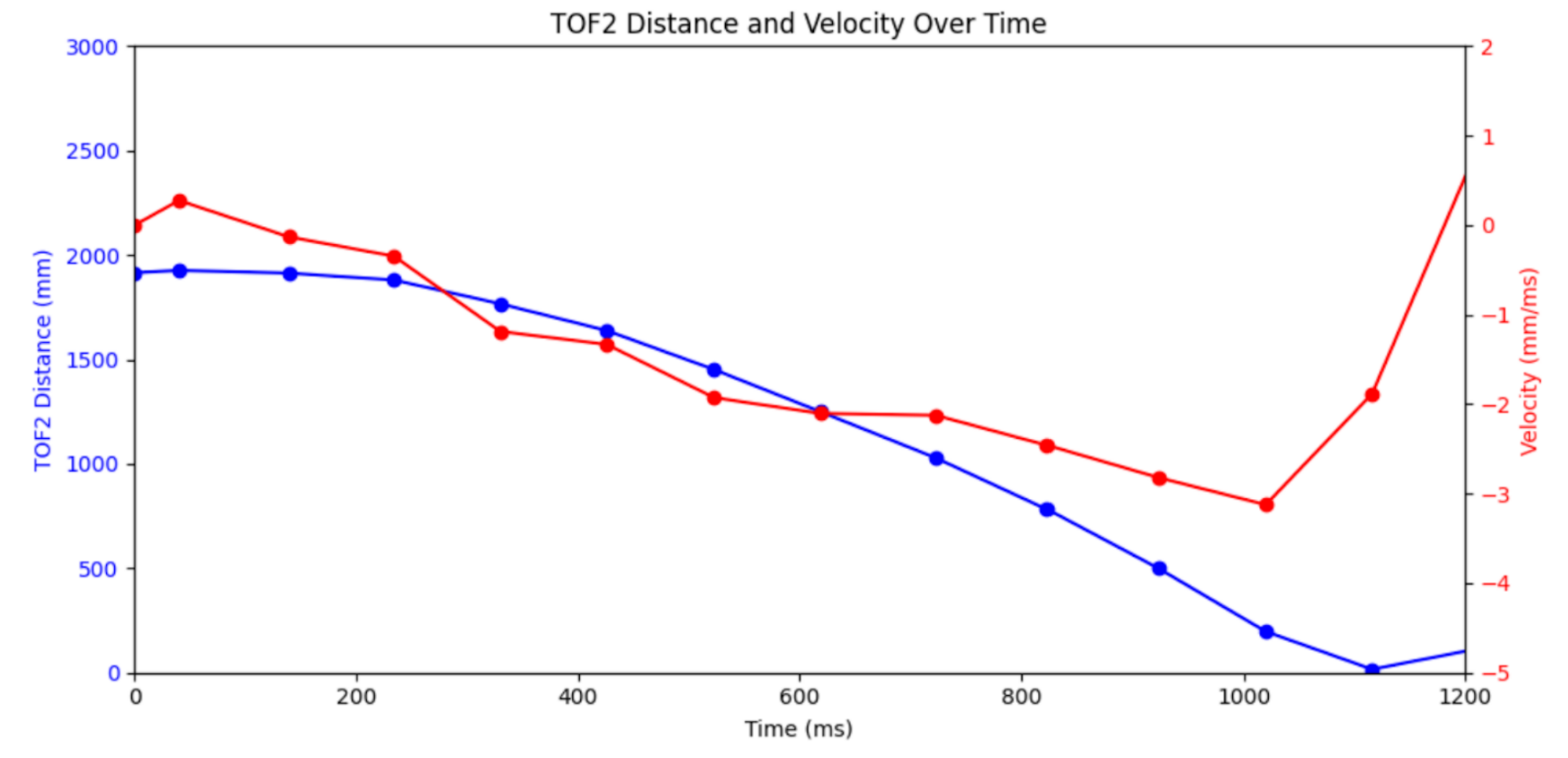
Close Test - **small correction, velocity units are in m/s
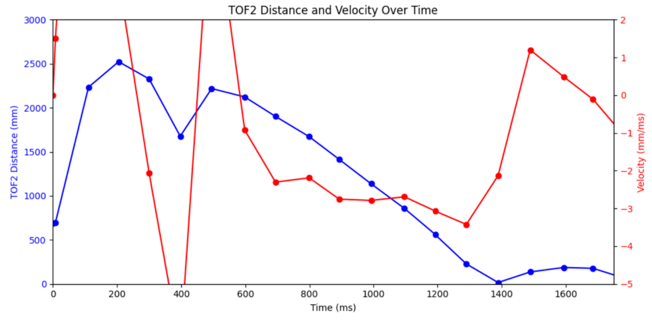
Mid Test - note the bad readings above 2000mm
Long Test - note the bad readings above 2000mm
Combining the velocity data from the valid parts of these trials into one comprehensive step response allowed me to get a better idea of how the car was slowing down:
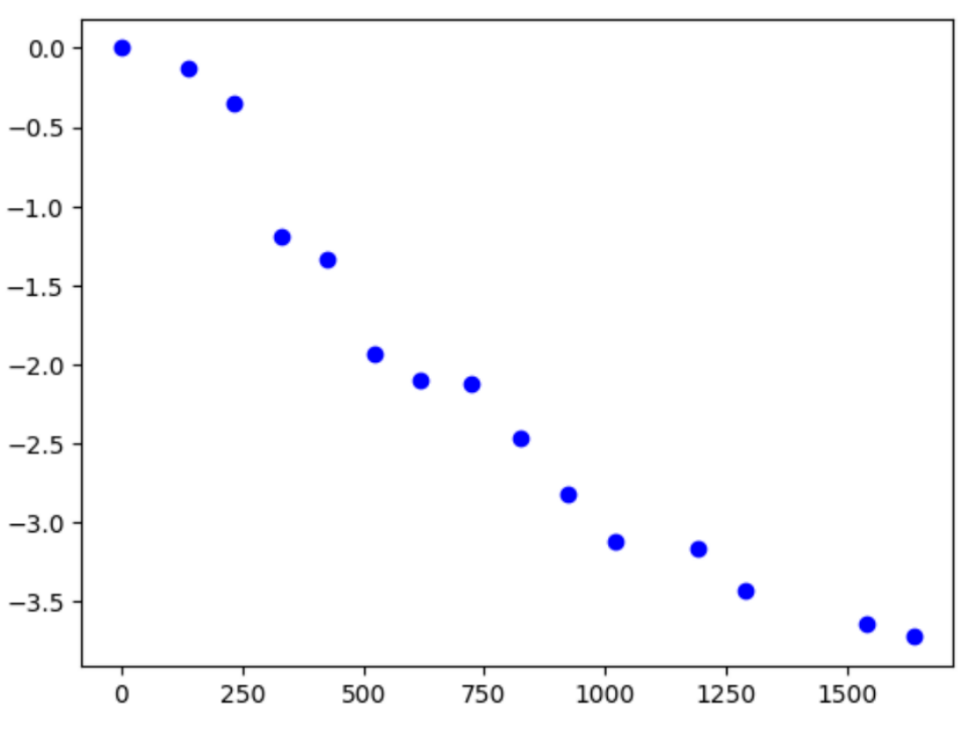
Combined Velocity Data - m/s vs ms
With this data, I then used the curve_fit function within the scipy.optimize module of scipy to fit an exponential decay curve to the data. Using this, I was able to find the steady state velocity, as well as the 90% rise time and velocity.
# Define the exponential decay function
def exponential_func(x, a, b, c):
    return a * np.exp(b * x) + c

# Fit the curve
popt, _ = curve_fit(exponential_func, combined_time, combined_velocity, p0=(1, -0.001, -3))
a, b, c = popt

# Generate fitted curve
x_fit = np.linspace(min(combined_time), max(combined_time) + 3000, 1000) # add 3000 to extend the graph beyond my data
y_fit = exponential_func(x_fit, *popt)

# Calculate Key Metrics
t0 = min(combined_time)
v0 = exponential_func(t0, *popt)
v_ss = c
v_90_decay = c + 0.1 * (v0 - c)
t_90 = np.log((v_90_decay - c) / a) / b
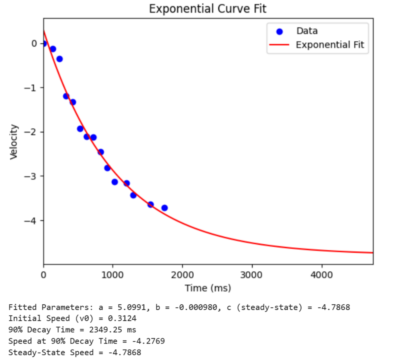
With these values, I then calculated d and m using the equations found above.
Simulating the Kalman Filter
In order to implement the Kalman Filter (KF) in python, I first transfered our dynamics into state space.
A = np.array([
    [0, 1],
    [0, d/m]
])

B = np.array([
    [0],
    [1/m]
])

C = np.array([[1, 0]])

x = np.array([[distance[0]], [0]]) # Initialize state vector
I then discretized the matrices. I used a dt of 100ms, because that matched my sensor speed pretty closely. I also defined the steady control input here.
Ad = np.eye(n) + dt * A
Bd = dt * B

u_ss = -1
Next I initialized my covariance matrices. I initially tried to use the formulas to calculate these, as well as referencing my lab 3 experimentation that found the standard deviation of the TOF sensor; however, I found trial and error to be the best method in this case.
# Process noise
sigma_1 = .10 # position variance
sigma_2 = 100 # speed variance

# Sensor noise
sigma_3 = 50

Sigma_u = np.array([[sigma_1**2, 0], [0, sigma_2**2]]) # confidence in model
Sigma_z = np.array([[sigma_3**2]]) # confidence in measurements
After defining all of the variables, I implemented the filter logic using the lecture example as a guide.
def kalman(mu, sigma, u, y, update = True):
    mu_p = Ad.dot(mu) + Bd.dot(u)
    sigma_p = Ad.dot(sigma.dot(Ad.transpose())) + Sigma_u
    if not update:
        return mu_p, sigma_p

    #run only if new measurement
    sigma_m = C.dot(sigma_p.dot(C.transpose())) + Sigma_z
    kkf_gain = sigma_p.dot(C.transpose().dot(np.linalg.inv(sigma_m)))

    y_m = y - C.dot(mu_p)
    mu = mu_p + kkf_gain.dot(y_m)
    sigma = (np.eye(2) - kkf_gain.dot(C)).dot(sigma_p)

    return mu, sigma

# Uncertainty for initial state
sigma = np.array([[20**2, 0], [0, 10**2]])

kf = []

i = 0
for t in time:
    # Step through discrete time
    update = time[i+1] <= t
    i += 1 if update else 0

    # Run Kalman filter for each time step
    x, sigma = kalman(x, sigma, u_ss, distance[i], update)
    kf.append(x[0])
When trusting the sensor measurements more than the process, the result was a filter that followed the data pretty closely. To much trust could lead to a filter at the mercy of sensor noise.
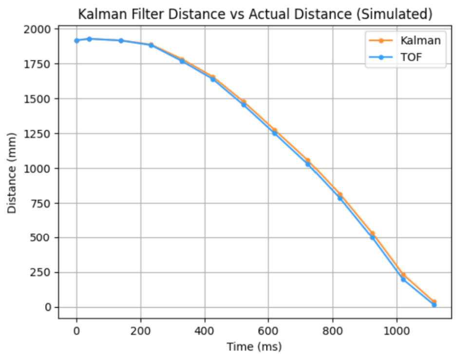
sigma_1 = 250, sigma_2 = 250, sigma_3 = 100
However, trusting the filter more lead to bigger discrepancies between the data and filter.
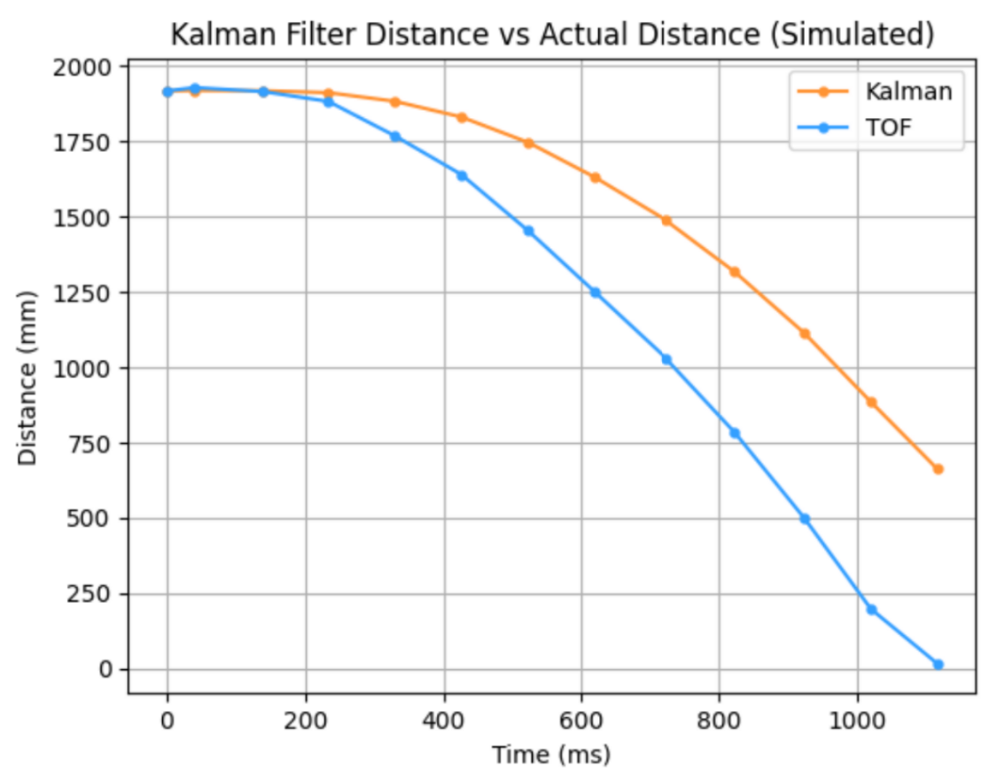
sigma_1 = 100, sigma_2 = 100, sigma_3 = 400
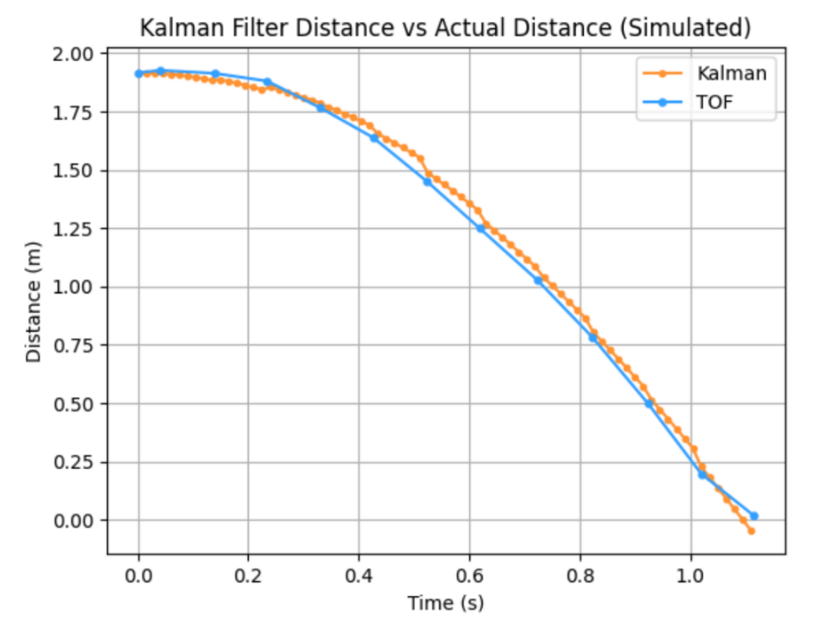
Interpolation
Running the KF at the speed of the TOF sensor works, but it doesn't really add much useful information for my robot's behavior. In order to be impactful, the KF needs to be able to run faster than the sensors, filling in the gaps between measurements with a more accurate model than just linear interpolation. To get this working in my simulator, I defined a higher resolution time span and looped through that instead. I also changed dt to 15ms to match the approximate speed of my PID loop on the artemis.
i = 0
interval = .015 # ms
steps = np.arange(0, (time[-1] ), interval)
for t in steps:
    # Step through discrete time
    update = time[i+1] <= t
    i += 1 if update else 0

    # Run Kalman filter for each time step
    x, sigma = kalman(x, sigma, u_ss, distance[i], update)
    kf.append(x[0])
Some debugging notes - I was running into some unit issues that would throw off my calculated dynamics. I fixed this by going through my entire setup and making sure every unit was unscaled (meters, seconds, kilograms only). Also, I found that setting the sensor uncertainty to an astronomically high number was a very useful debugging step. This meant the filter would ignore the sensor data, and I could get a good idea of the motion that the filter would predict using just the system dynamics and control input.
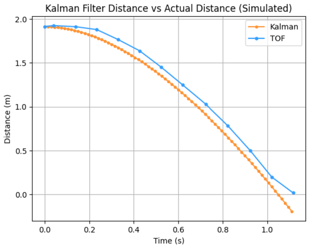
Note how the filter completely ignores the sensor data. This filter is pretty well tuned, as the predicted motion mostly matches the actual motion even without any actual fusion between the two.
Implementation On My Robot
When sending the BLE command to my car, I made sure to make all of the tunable parameters changeable on the python side. This made tuning much quicker, as I didn't have to upload new artemis code for small changes.
kp = 0.1
ki = 0
kd = .004


target = 300 # [mm]


d = -0.209
m = 0.213
uf = 1000 # control input scale factor

sig1 = .10
sig2 = 100
sig3 = 50

runtime = 6000 # [ms]
The logic of the KF didn't change - it just needed to be refactored for matrix operations in C. The general structure was a BLE command that sends all of the parameters; within this command a loop runs that repeatedly calls functions that collect data (TOF), predict motion (KF), and calculate/send control inputs (PID).
I also made use of global variables whenever possible to simplify the arguments passed between functions.
I implemented this with the KF interpolating between measurements, allowing the robot to adjust control inputs very quickly (the speed of the loop was about 10ms).
while (millis() - start_time < runtime) //run for a fixed amount of time
{

    // attempt to refresh sensor data
    if ( (tof1Counter < MAX_TIME_STAMPS) && (tof2Counter < MAX_TIME_STAMPS)  )
        {
        collect_tof();
        }

    // predict new distance value
    kalman(x, sigma, Ad, Bd, Sigma_u, Sigma_z, C, uf);
    float current_distance = tof_kalman[pidCounter];

    // calculate error
    float error = current_distance - target;
    float prev_error = tof_kalman[pidCounter-1] - target;

    // calculate PID input and send to motors
    pid_control_input[pidCounter] = send_control_input(kp, ki, kd, error, prev_error, df_alpha);

    // update time array + counter
    pid_time_stamps[pidCounter] = millis();
    pidCounter = pidCounter + 1;

}
When tuning my controller, there were many parameters to consider:
Kp and Kd (I left out an integrator term for this lab; ess was low). The gains had the same effect as in the previous PID lab. The added challenge was that each time a new sensor value came in, the filtered data would jump to adjust to this, causing a derivative spike. I added a LPF to deal with this noise.
Measurement uncertainty. Lowering the sensor uncertainty led to a filter that followed the TOF sensors very closely - making this too low would mean the filter was subject to the same noise as the sensors. Too high, and the filter may drift too far away from the actual values.
Process uncertainty. Sig1 and sig2 represent the uncertainty in the process model for position and velocity, respectively. Low values for these parameters indicate high confidence in the model's predictions, causing the filter to rely more on its internal dynamics and respond less to sensor updates. High values signal low trust in the model, making the filter lean more heavily on sensor measurements. Risks and benefits of over/undertuning are similar to that of measurement uncertainty.
m and d. While these terms were estimated from experimental trials, they could still be tweaked. A larger m meant that the dynamics represented a car with more inertia - a control input would accelerate the car less. d plays more of a role scaling the maximum velocity and also how quickly speed decays when a control input is removed.
u. While the control input comes from the PID controller and probably should not technically be changed, I found it an easy "hack" for getting closer to my desired filter behavior. This could probably be replicated by tweaking m and d, or perhaps I have a unit issue. However, I added a standalone scaling factor to my control input - it still came from my controller, but I just found that amplifying its value allowed it to have the desired effect on the predicted trajectory.
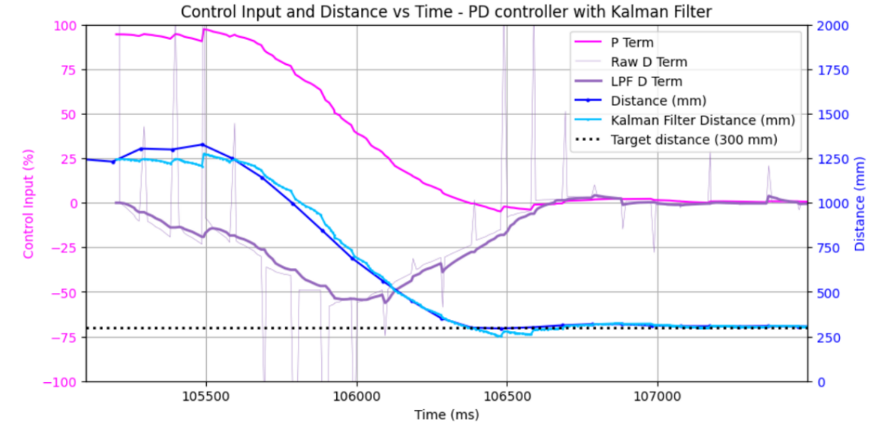
With all of this in mind, I spent some time tuning my controller and KF. This was my final result:
Collaboration
I worked with Jack Long and Lucca Correia extensively. I also referenced Stephan Wagner's site for sense checking my uncertainty values. Lastly, ChatGPT helped me make pretty plots and initialize matrices correctly in C.