PID Orientation Control

To ensure even angular spacing between readings, I utilized my orientation PD controller from lab 6. I made one small change to the command: from my laptop I sent a target_increment and time_increment variable. The target for the controller would increase by target_increment every time time_increment seconds passed. I eventually settled on an increment of 16 degrees every second, which was a big enough change for the robot, while still giving good resolution in the data. Other than this change, my implementation of orientation control was reused from lab 6 - with some tweaking of the gains, my robot was able to take stable, incremented steps in orientation. I chose to keep my TOF sensor running as fast as possible in order to collect as much data as possible. The increment sizes I chose correspond to about 26 fixed orientations per rotation, but the fast speed of my TOF sensor and the slow speed of my rotation meant that I was able to collect good data between set points as well.

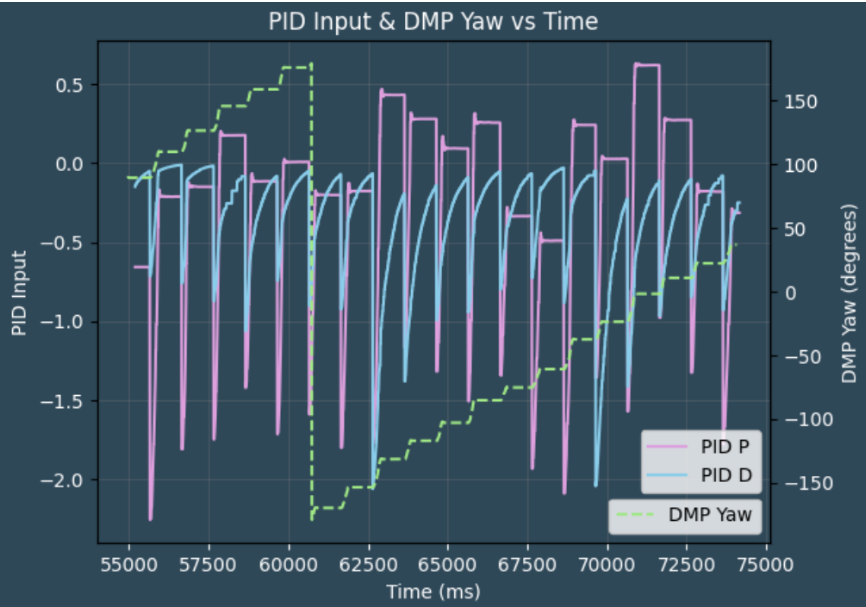
The figure above shows the PID P and D terms along with the DMP yaw over time (kp = 0.1, kd = 0.025). Each sharp step in yaw corresponds to one complete orientation increment, and the smooth decay of PID values after each step confirms controlled movement.

I also had the artemis log the current orientation every time a TOF data point was collected. This made plotting data straightforward:

    tof2_array[tof2Counter] = distance2 ;
    tof2_orientation[tof2Counter] = dmp_yaw_array[dmpCounter-1];
    tof2Counter = tof2Counter + 1;

I used the DMP data rather than assuming that each fixed point would be perfectly spaced across a full rotation. This is because my PD controller has no integrator term to eliminate steady state error - luckily this issue is easily avoided by using the accurate DMP data for orientation.

Local Polar Scans

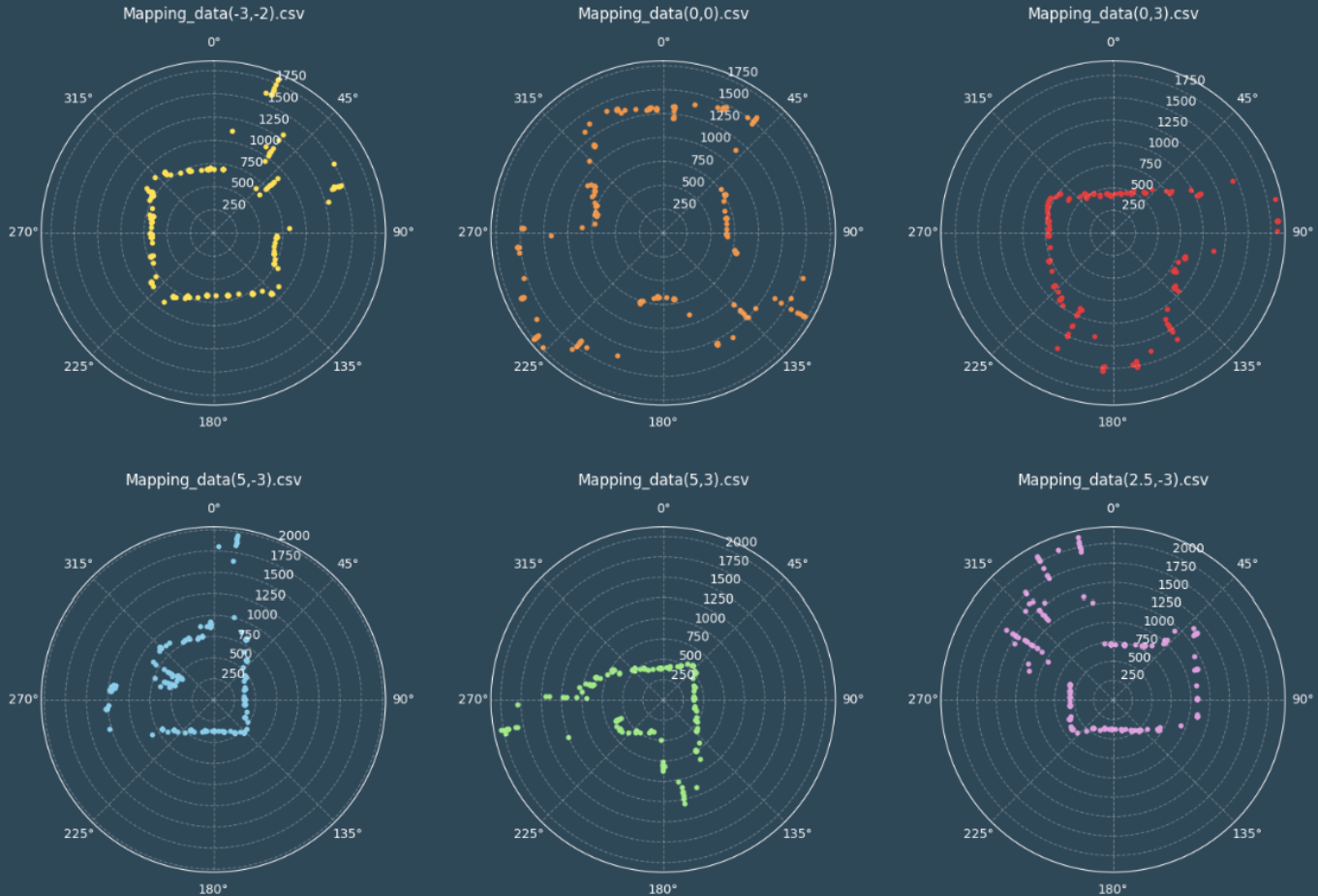
Each scan was performed with the robot spinning on-axis at one of the following positions (in feet):
(-3, -2), (0, 0), (0, 3), (5, -3), (5, 3)

After each rotation, I plotted the TOF values against orientation to verify consistency. Polar plots from each location clearly outline local environmental features, and points that overlap across multiple rotations line up. The biggest drift I measured during collection was half an inch, but it was usually less than this. This means that I would expect my measurements to be accurate to around half an inch at worst - pretty good for a 4m x 4m space. On average, this error will be closer to roughly 1/4".

At this point, I was also realizing that my TOF sensor was struggling with distances above 1000mm. I felt that one of the corners of the enviroment was severely uncaptured, so I took an extra measurement from (2.5, -3).

Merging into Global Frame

With all of the data collected, I used transformation matrices to convert each scan's local polar coordinates into global Cartesian coordinates. Refering to Farrell's Lecture on T-matrices, each point was rotated and translated based on the robot's scan position and orientation. Something that made this step easier was the fact that I started my robot facing north for each scan, aligning all of my rotational data.

    distance_ft = row["TOF2 Value"] * MM_TO_FT
    theta = np.deg2rad(orientation_deg)
    

    # Transformation matrix using current theta
    T = np.array([
        [np.cos(theta), -np.sin(theta), x_robot],
        [np.sin(theta),  np.cos(theta), y_robot],
        [0,              0,             1]
    ])

    # Local point is (TOF + offset, 0, 1)
    P_local = np.array([
        [distance_ft + sensor_offset],
        [0],
        [1]
    ])

    # Transform to global coordinates
    P_global = T @ P_local

I measured the sensor offset to be 3 inches for my robot - I defined this to be in the x direction relative to my robot. I then plotted all of the transformed data together:

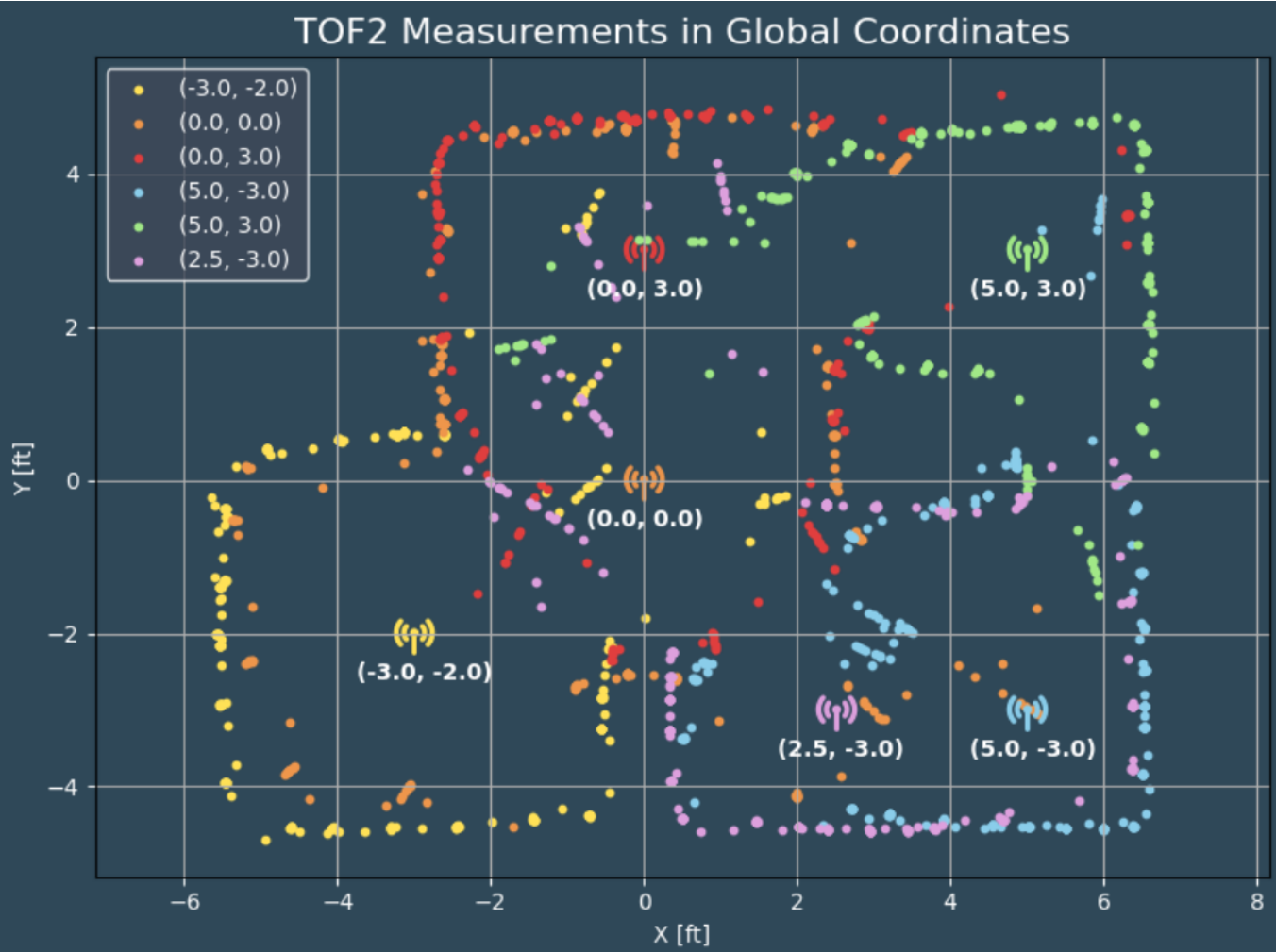
Walls

To obtain a complete map of the enviroment, I estimated straight-line segments that connected clusters of points.

    starts = [
    (-5.5, -4.6), (-5.5,  0.3),
    (-2.6,  0.6), (-2.6,  4.5),
    ( 6.6,  4.6), ( 6.4, -4.4),
    ( 0.5, -4.5), ( 0.4, -2.4),
    (-0.4, -2.4), (-0.4, -4.4),
    ( 2.6, -0.4), ( 2.5,  1.6),
    ( 4.4,  1.5), ( 4.4, -0.4)
    ]

    ends = [
    (-5.5,  0.3), (-2.6,  0.6),
    (-2.6,  4.5), ( 6.6,  4.6),
    ( 6.4, -4.4), ( 0.5, -4.5),
    ( 0.4, -2.4), (-0.4, -2.4),
    (-0.4, -4.4), (-5.5, -4.6),
    ( 2.5,  1.6), ( 4.4,  1.5),
    ( 4.4, -0.4), ( 2.6, -0.4)
    ]

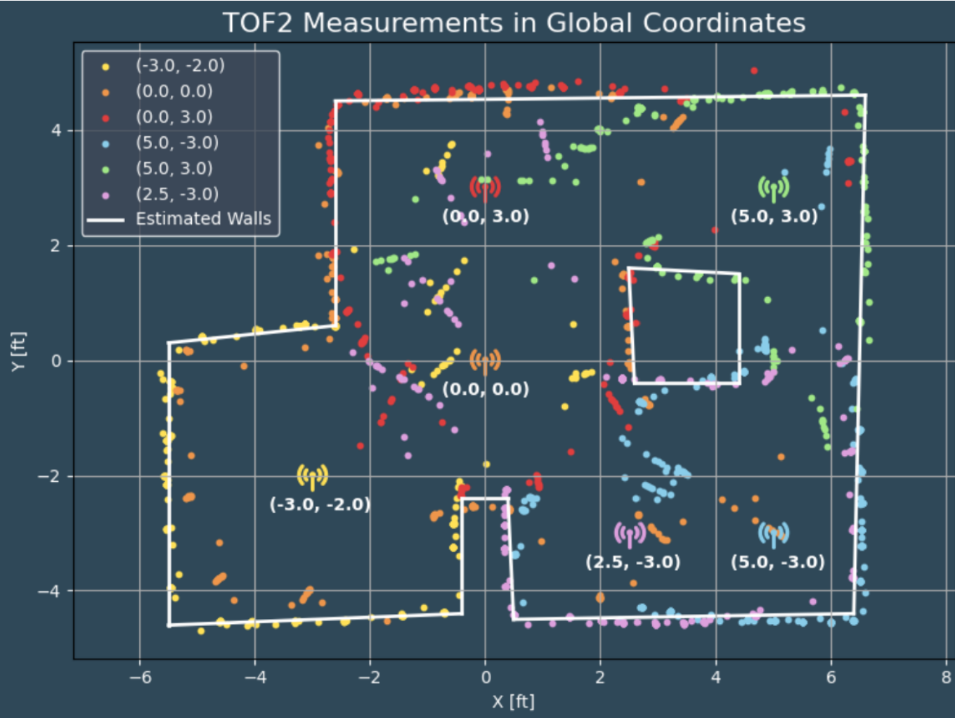Whenever my sensor was pointed at a surface more than 1000mm away, it would take a spread of noisy data. This is especially visible in the central regions of the environment, as the scans taken from the edge would collect poor data when pointing towards the open center. For this reason, when drawing my lines I prioritized data taken from a short distance, and did my best to ignore the noise in the middle. I can also see that my additional scan helped add fidelity to my map in the bottom central region.

Some of the lines are slanted/misproportioned. There are many possible causes for these discrepancies:

• The environment itself was not perfectly aligned with the grid
• Drift during a scan
• TOF sensor noise
• Yaw drift in the DMP data
• I oriented the robot slightly misaligned with north at the beginning

I made a few manual adjustments to correct for some of this, but I mostly trusted the data. This final map will be used in lab 10 for localization!

Collaboration

I worked with Jack Long and Lucca Correia on this lab. ChatGPT helped make my plots more readable.